Chapter 22 Examples of PLS regression with agroclimatic metrics
Learning goals for this lesson
- Get an overview of studies that have been using the PLS approach with agroclimatic metrics
- Get a feeling for the effectiveness of the approach across locations and species
- Start thinking about possible limitations of this approach in delineating temperature response phases
22.1 PLS regression across species and agroclimatic contexts
Since 2012, PLS regression using agroclimatic metrics (chill and heat) as inputs has been applied in a bunch of different contexts. The method has been adopted by a few other researchers as well, but I’ll restrict the examples for this chapter to the studies that I was involved in.
22.1.1 Chestnut, jujube and apricot in Beijing
One of the coldest locations we’ve used this approach in is Beijing, where, led by Guo Liang we worked with bloom data for Chinese chestnut (Castanea mollissima) and jujube (Ziziphus jujuba) to delineate chilling and forcing periods (Guo, Dai, Ranjitkar, et al. 2014). In another study, we also examined datasets for apricot (Prunus armeniaca) and mountain peach (Prunus davidiana). Here are the results:
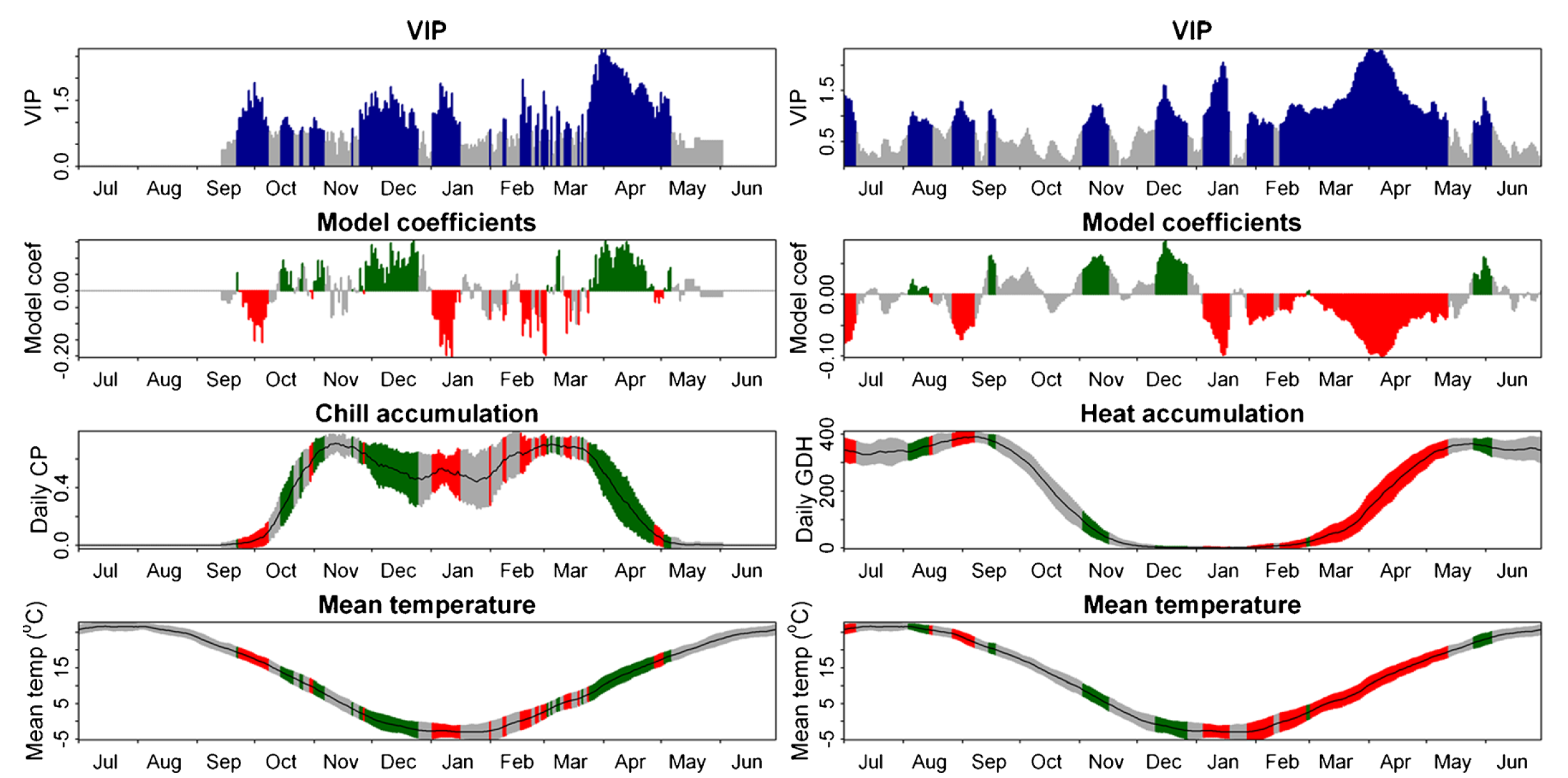
Results of a PLS analysis based on the relationship between daily chill (quantified with the Dynamic Model) and heat (quantified with the GDH model) accumulation and bloom of Chinese chestnut (Castanea mollissima) in Beijing, China (Guo, Dai, Ranjitkar, et al. 2014)
Results of a PLS analysis based on the relationship between daily chill (quantified with the Dynamic Model) and heat (quantified with the GDH model) accumulation and bloom of jujube (Ziziphus jujuba) in Beijing, China (Guo, Dai, Ranjitkar, et al. 2014)
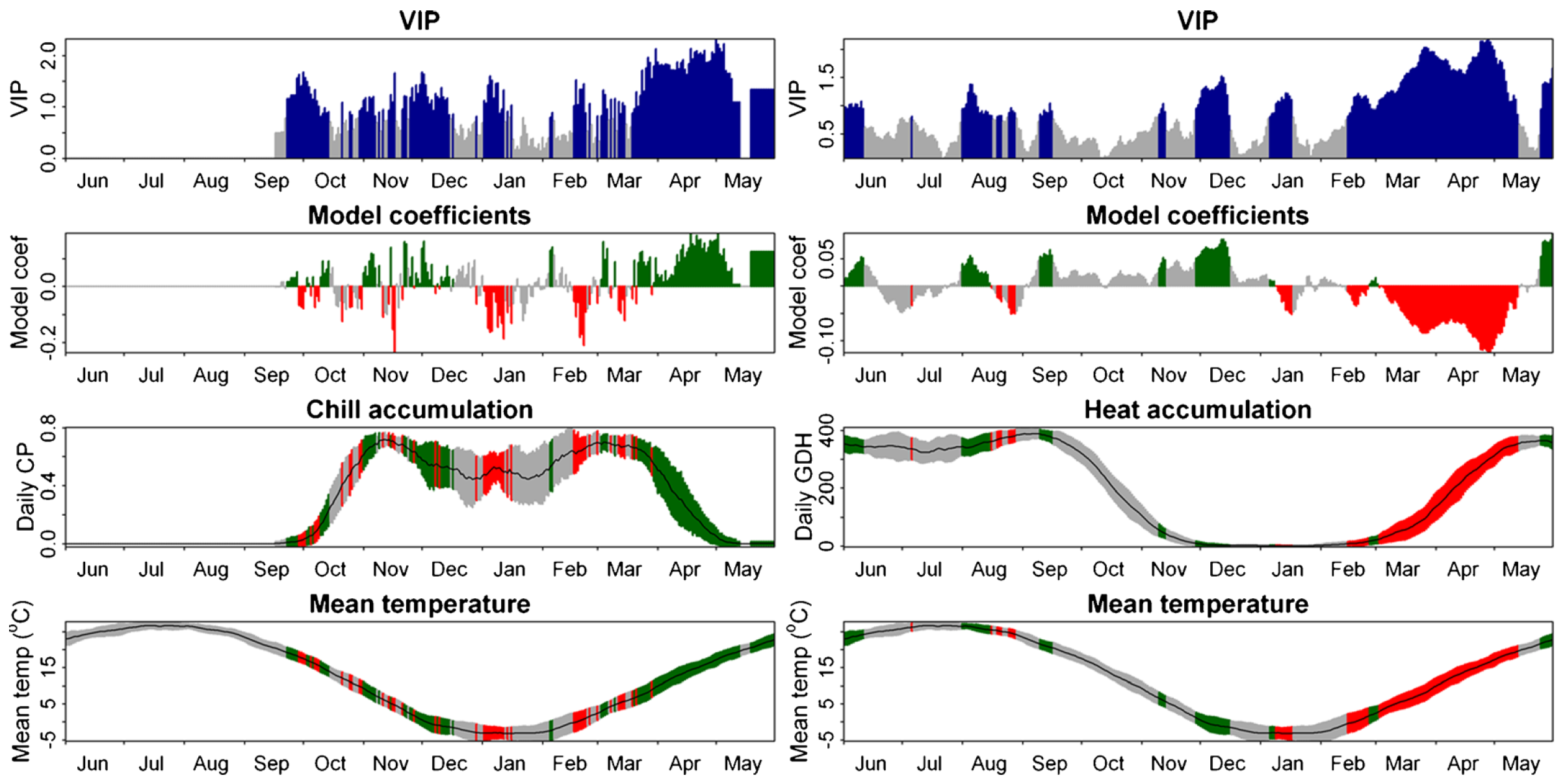
Results of a PLS analysis based on the relationship between daily chill (quantified with the Dynamic Model) and heat (quantified with the GDH model) accumulation and bloom of mountain peach (Prunus davidiana) in Beijing, China (Guo, Luedeling, et al. 2014)
Results of a PLS analysis based on the relationship between daily chill (quantified with the Dynamic Model) and heat (quantified with the GDH model) accumulation and bloom of apricot (Prunus armeniaca) in Beijing, China (Guo, Luedeling, et al. 2014)
For apricots, we also ran PLS regressions with multiple chill metrics, i.e. Chilling Hours, the Utah Model (Chill Units) and the Dynamic Model (Chill Portions):
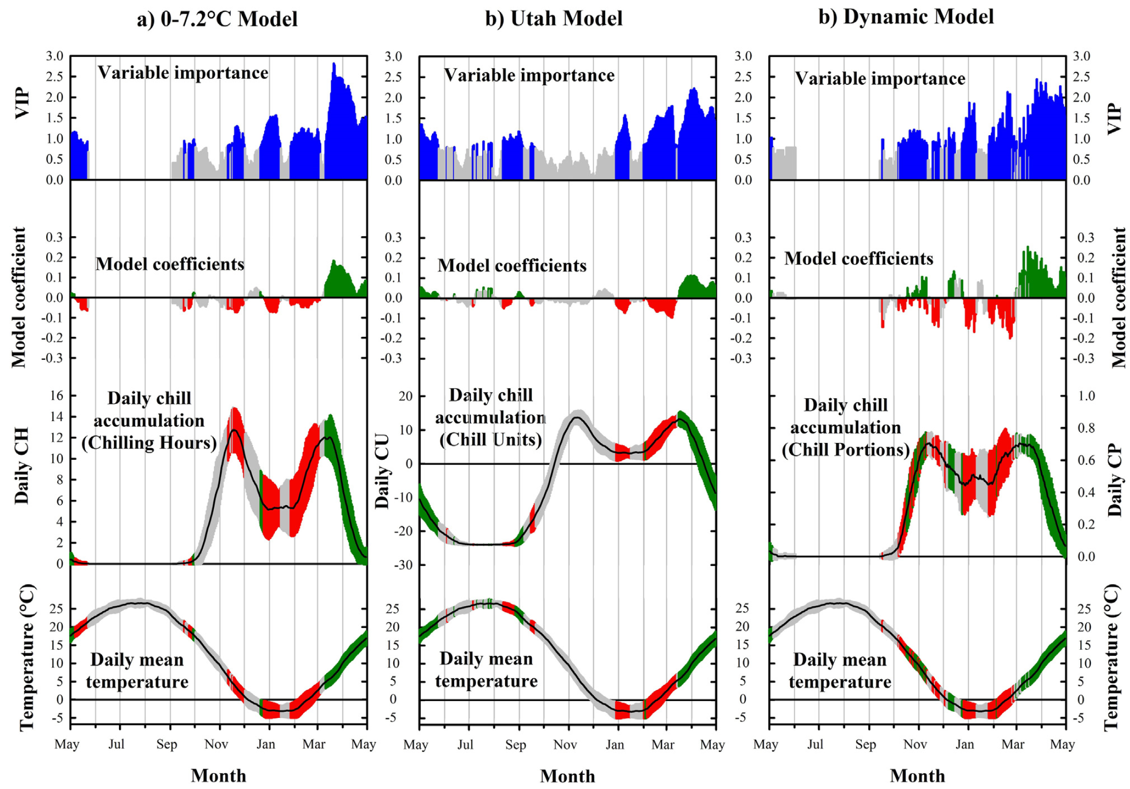
Results of a PLS analysis based on the relationship between daily chill and heat accumulation and bloom of apricot (Prunus armeniaca) in Beijing, China. Coefficients for heat are not shown here (they are similar to what’s shown in the previous figure). Chill accumulation was quantified with the Chilling Hours Model (left), the Utah Model (middle) and the Dynamic Model (right) (Guo, Xu, et al. 2015)
In all analyses of phenology records from Beijing, the forcing period was easy to delineate, but the chilling period was difficult to see.
22.1.2 Apples in Shaanxi Province, China
Guo Liang also led a study on apple phenology in Shaanxi, one of China’s main apple growing provinces:
Results of a PLS analysis of the relationship between chill (in Chill Portions) and heat (in GDH) and bloom dates of apple in Shaanxi, China (Guo et al. 2019)
Also here the chilling phase was visible but difficult to delineate.
22.1.3 Cherries in Klein-Altendorf
Winters in Beijing and Shaanxi are rather cold. Let’s look at a slightly warmer location - cherries in Klein-Altendorf.
Results of a PLS analysis of bloom dates of cherries ‘Schneiders späte Knorpelkirsche’ in Klein-Altendorf, Germany, based on chill (in Chill Portions) and heat (in GDH) accumulation (Luedeling, Guo, et al. 2013)
Again, it’s pretty difficult to see the chilling period.
22.1.4 Apricots in the UK
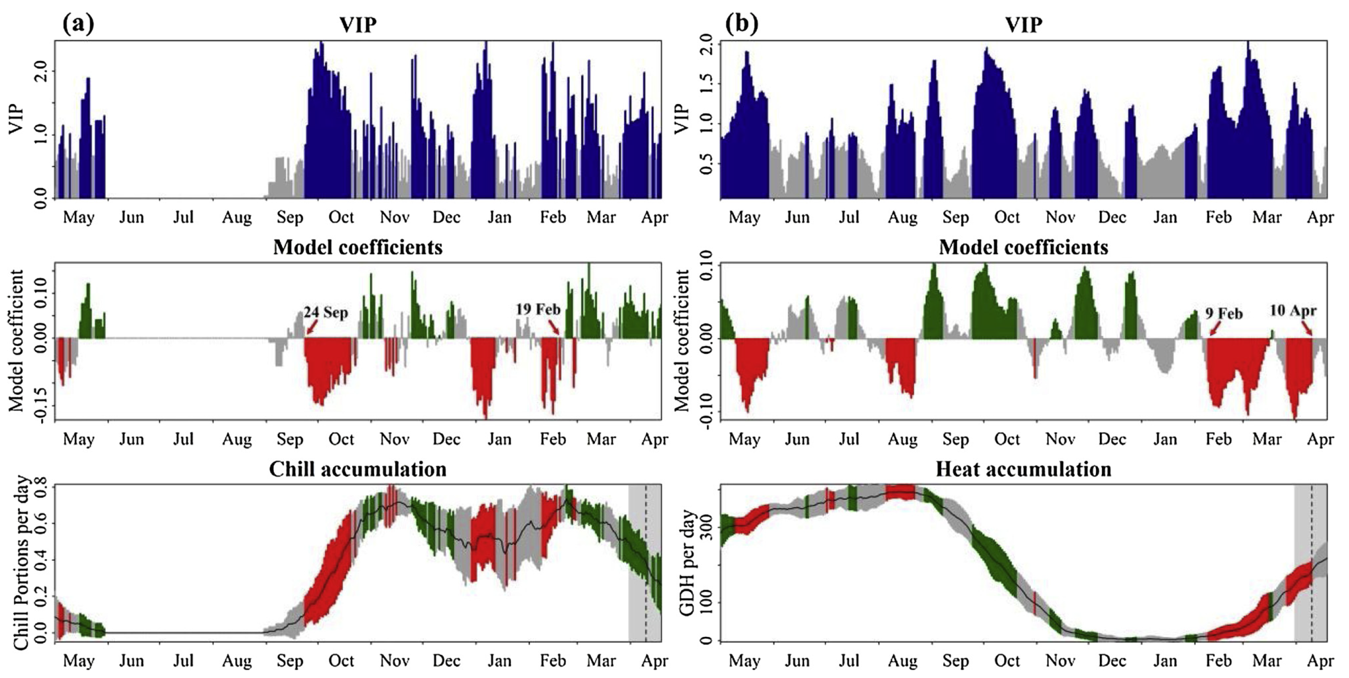
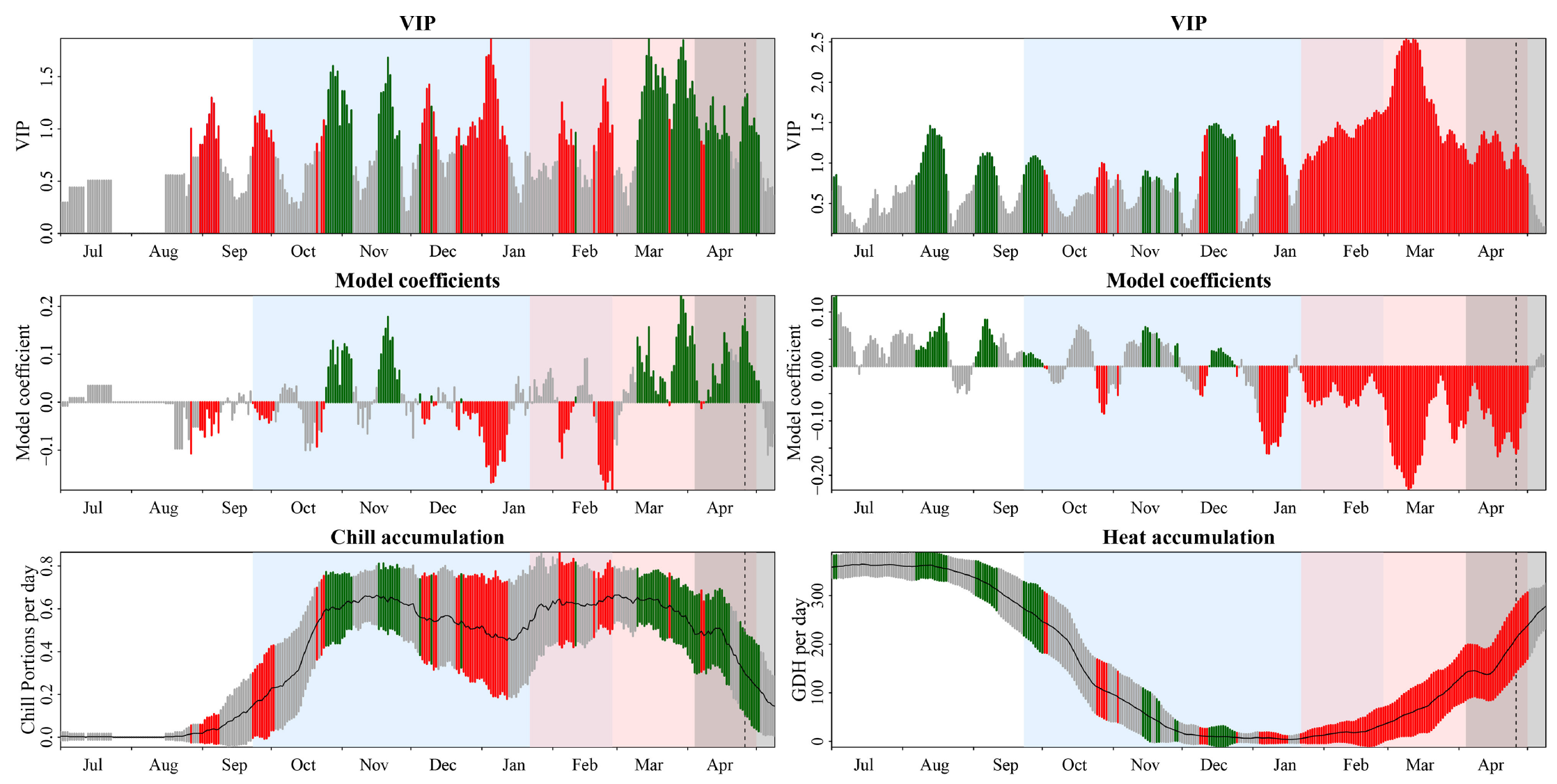
For apricots in the UK National Fruit Collection at Brogdale Farm in Faversham, southern England, we can see a clear chill response phase in January and February, but this period is quite a bit later than we would normally expect chill accumulation to start:
Results of a PLS analysis of apricot bloom in the southern UK, based on chill accumulation (in Chill Portions) and heat accumulation (in GDH) (Martı́nez-Lüscher et al. 2017)
22.1.5 Grapevine in Croatia
Grapes also have chilling requirements, so Johann Martínez-Lüscher, who also led the UK apricot study, looked into the temperature response of grapes grown in Croatia:
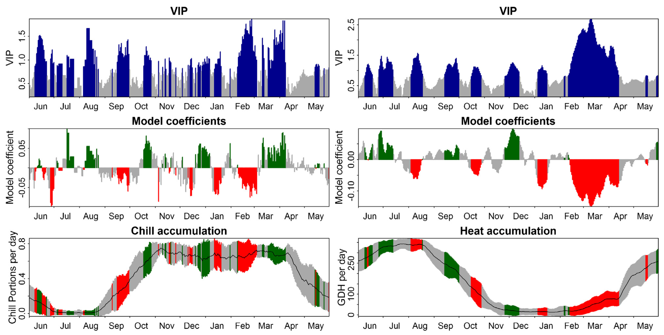
Results of a PLS analysis of flowering dates of grapevine (cv. ‘Riesling Italico’) in Mandicevac, Croatia. Chill was quantified with the Dynamic Model, heat with the Growing Degree hours Model (Martı́nez-Lüscher et al. 2016)
Here in Croatia, where winters are warmer than in the earlier locations and chill accumulation rates are more variable, we see the chilling period emerging more clearly, with a particularly pronounced bloom response to chill accumulation in December and January. If we choose to be a bit more generous in our interpretation, we can see a chilling period extending from late September to February.
22.1.6 Walnuts in California
Let’s look at a location with an even warmer winter. For walnuts in California, we could already see the chilling period when working with raw temperatures, and we can also see it clearly when we use agroclimatic metrics:
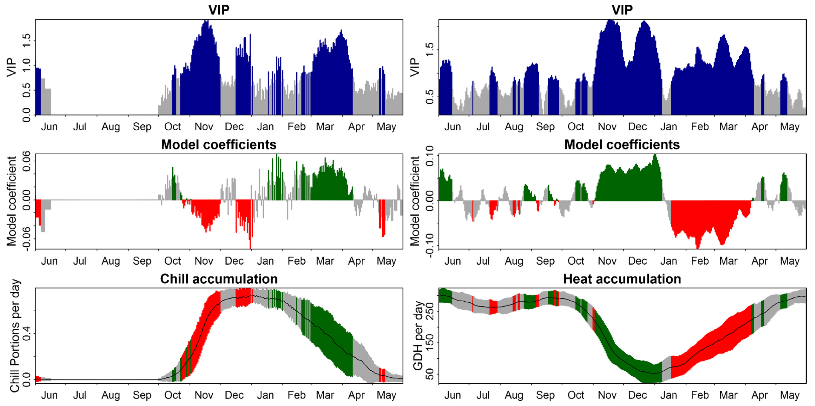
Results of a PLS analysis of leaf emergence dates of walnuts (cv. ‘Payne’) in Davis, California. Chill was quantified with the Dynamic Model, heat with the Growing Degree Hours Model (Luedeling, Guo, et al. 2013)
Once again, we can see the chilling period pretty clearly in this analysis. As we’ve seen before, it appears to consist of two parts (what could be the reason for this? May be worth looking into at some point), but we can easily spot a period between mid-October and the end of December, during which bloom dates respond to high chill accumulation rates.
22.1.7 Almonds in Tunisia
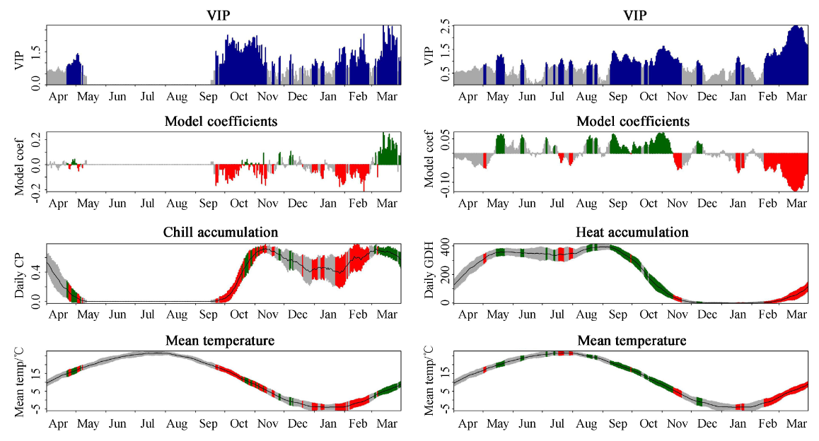
Sfax in Central Tunisia is an even warmer location - close to the margin of deciduous nut cultivation. In a study led by Haïfa Benmoussa, we evaluated bloom data of a total of 37 almond cultivars. In virtually all cases, we could clearly delineate both the chilling phase and the forcing period. The following three figures show the results.
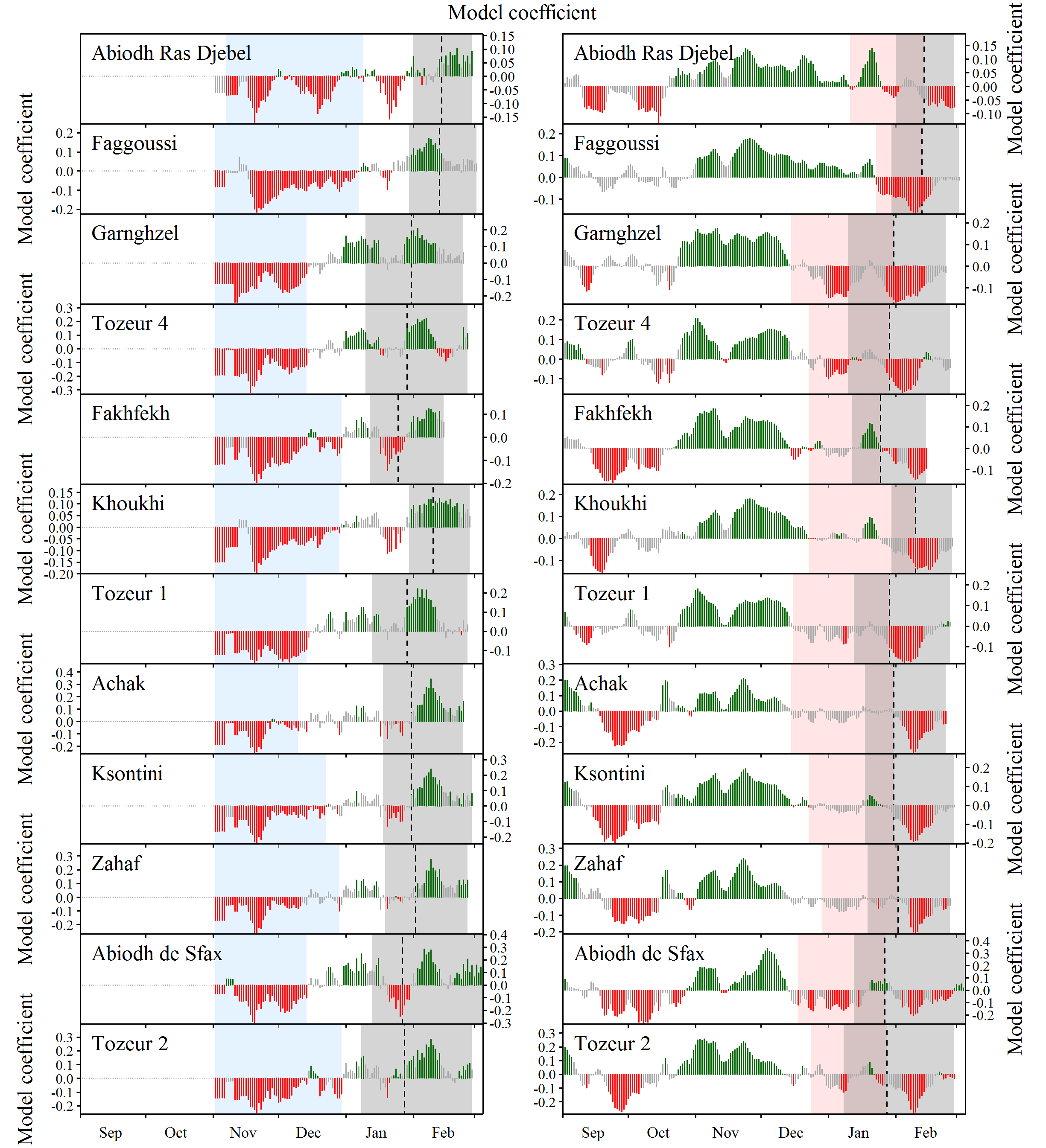
PLS results for almond cultivars near Sfax, Tunisia - part 1 (Haı̈fa Benmoussa et al. 2017)

PLS results for almond cultivars near Sfax, Tunisia - part 2 (Haı̈fa Benmoussa et al. 2017)
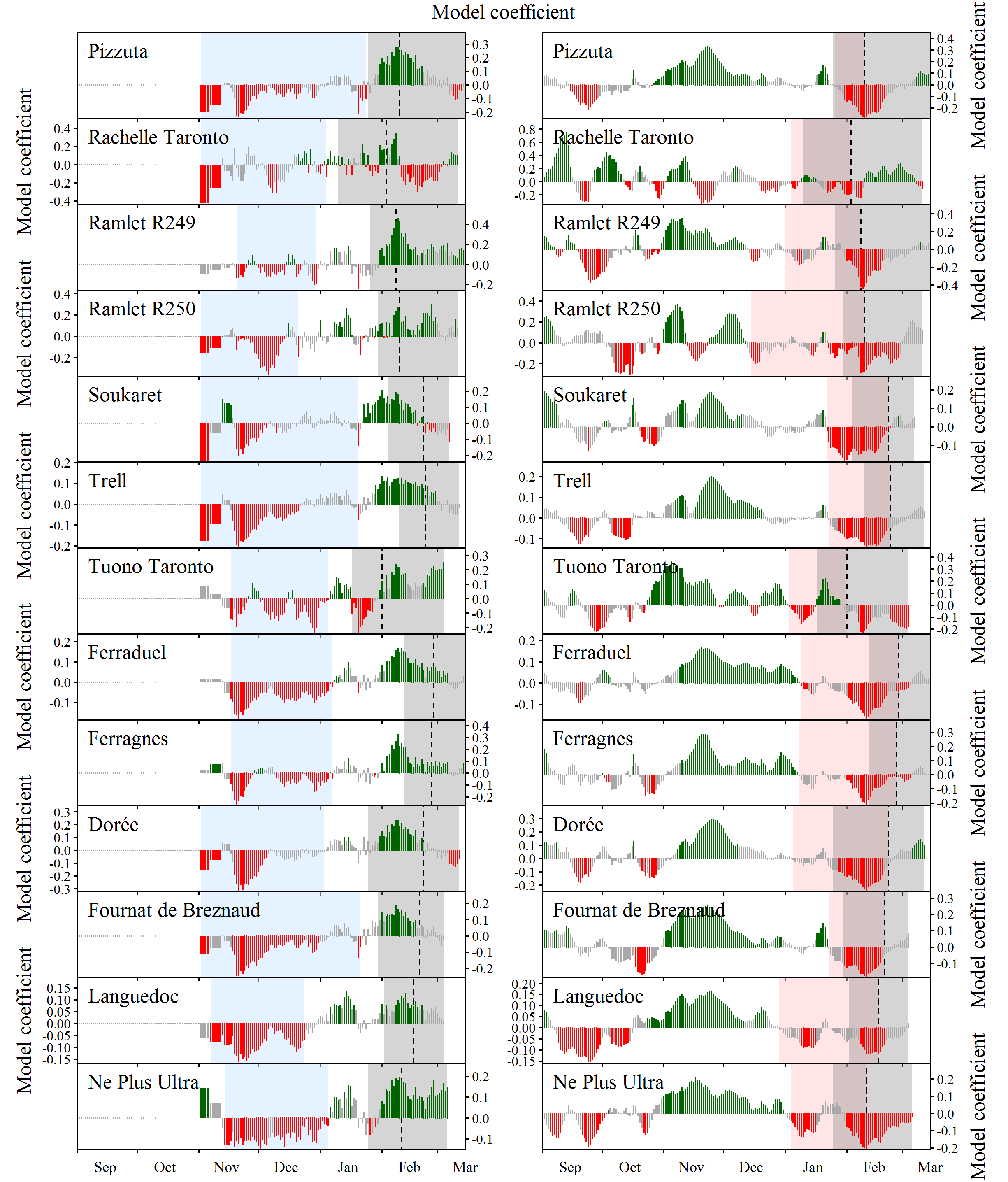
PLS results for almond cultivars near Sfax, Tunisia - part 3 (Haı̈fa Benmoussa et al. 2017)
22.1.8 Pistachios in Tunisia
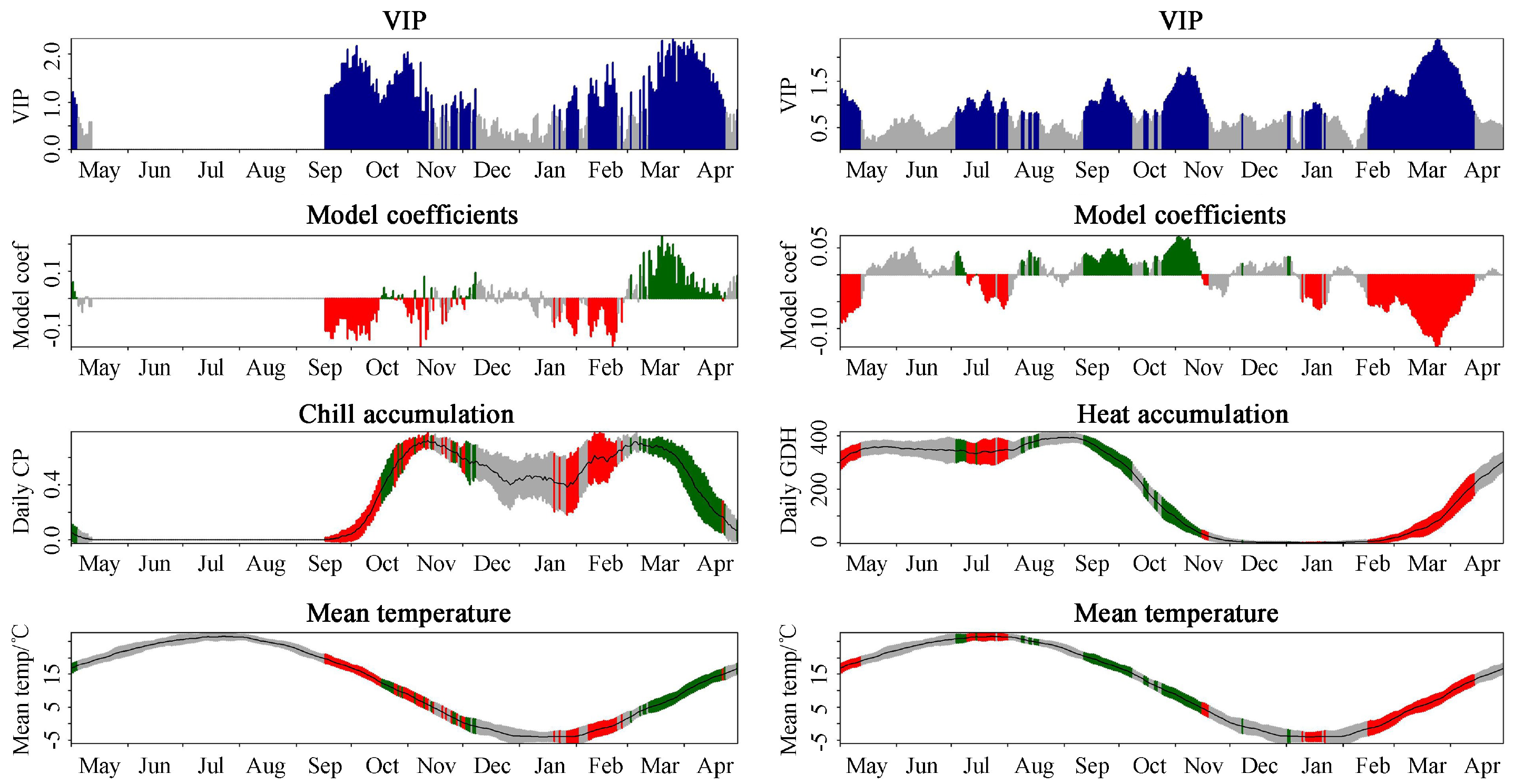
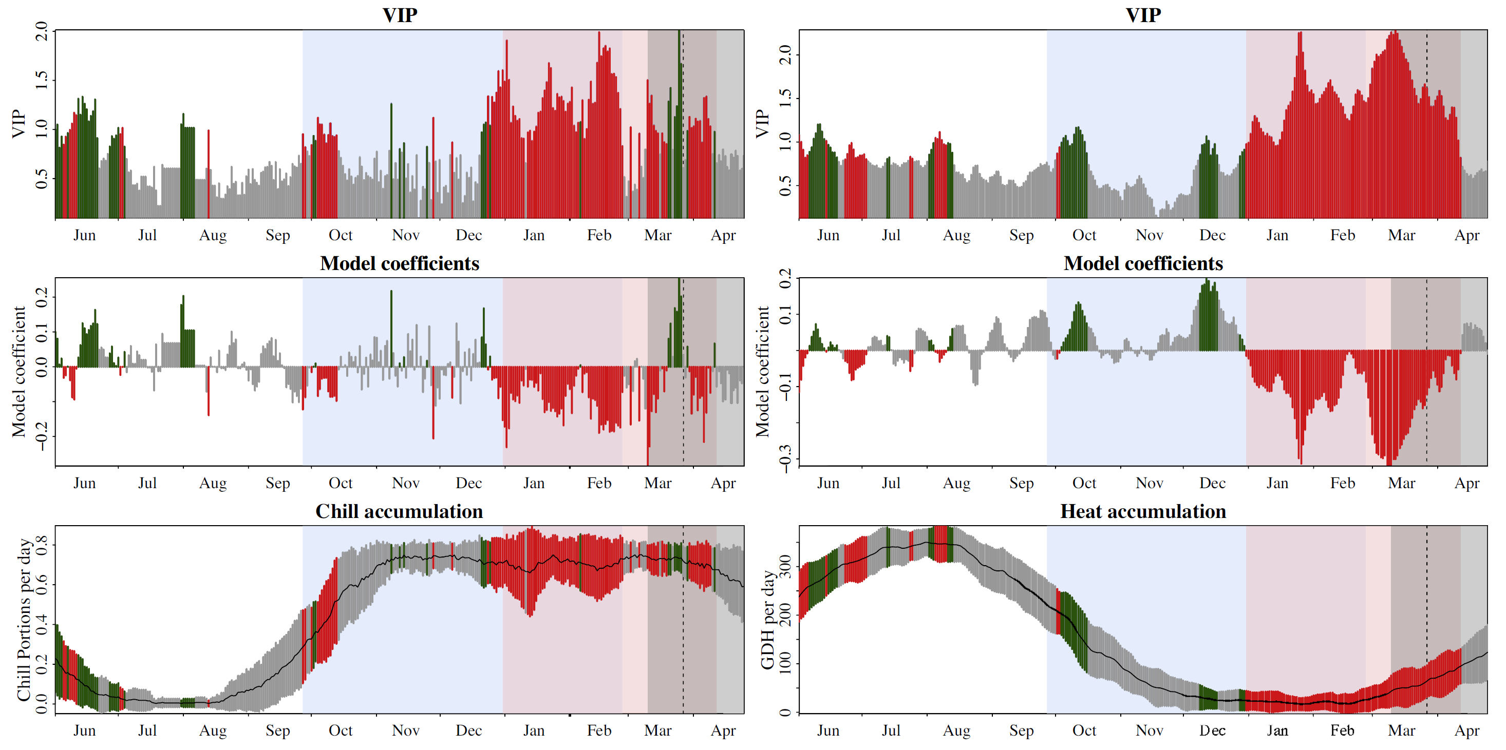
We also evaluated data for pistachios from the same experimental station in the Sfax region of Tunisia. For this crop, we found a long chilling period, with very clear responses to chill accumulation rates. Interestingly, the forcing period was now hard to see:

PLS results for pistachios near Sfax, Tunisia (Haïfa Benmoussa et al. 2017)
Exercises on examples of PLS regression with agroclimatic metrics
Please document all results of the following assignments in your learning logbook.
- Look across all the PLS results presented above. Can you detect a pattern in where chilling and forcing periods could be delineated clearly, and where this attempt failed?
- Can you think about possible reasons for the success or failure of PLS analysis based on agroclimatic metrics (if so, write down your thoughts)?
References
Benmoussa, Haı̈fa, Mohamed Ghrab, Mehdi Ben Mimoun, and Eike Luedeling. 2017. “Chilling and Heat Requirements for Local and Foreign Almond (Prunus dulcis Mill.) Cultivars in a Warm Mediterranean Location Based on 30 Years of Phenology Records.” Agricultural and Forest Meteorology 239: 34–46. https://doi.org/10.1016/j.agrformet.2017.02.030.
Benmoussa, Haïfa, Eike Luedeling, Mohamed Ghrab, Jihène Ben Yahmed, and Mehdi Ben Mimoun. 2017. “Performance of Pistachio (Pistacia vera L.) in Warming Mediterranean Orchards.” Environmental and Experimental Botany 140 (August): 76–85. https://doi.org/10.1016/j.envexpbot.2017.05.007.
Guo, Liang, Junhu Dai, Sailesh Ranjitkar, Haiying Yu, Jianchu Xu, and Eike Luedeling. 2014. “Chilling and Heat Requirements for Flowering in Temperate Fruit Trees.” International Journal of Biometeorology 58 (6): 1195–1206. https://doi.org/10.1007/s00484-013-0714-3.
Guo, Liang, E Luedeling, Jun-Hu Dai, and Jian-Chu Xu. 2014. “Differences in Heat Requirements of Flower and Leaf Buds Make Hysteranthous Trees Bloom Before Leaf Unfolding.” Plant Diversity and Resources 36 (2): 245–53. https://doi.org/10.7677/ynzwyj201413081.
Guo, Liang, Jinghong Wang, Mingjun Li, Lu Liu, Jianchu Xu, Jimin Cheng, Chengcheng Gang, et al. 2019. “Distribution Margins as Natural Laboratories to Infer Species’ Flowering Responses to Climate Warming and Implications for Frost Risk.” Agricultural and Forest Meteorology 268: 299–307. https://doi.org/10.1016/j.agrformet.2019.01.038.
Guo, Liang, Jianchu Xu, Junhu Dai, Jimin Cheng, and Eike Luedeling. 2015. “Statistical Identification of Chilling and Heat Requirements for Apricot Flower Buds in Beijing, China.” Scientia Horticulturae 195: 138–44. https://doi.org/10.1016/j.scienta.2015.09.006.
Luedeling, Eike, Liang Guo, Junhu Dai, Charles Leslie, and Michael M Blanke. 2013. “Differential Responses of Trees to Temperature Variation During the Chilling and Forcing Phases.” Agricultural and Forest Meteorology 181: 33–42. https://doi.org/10.1016/j.agrformet.2013.06.018.
Martı́nez-Lüscher, Johann, Paul Hadley, Matthew Ordidge, Xiangming Xu, and Eike Luedeling. 2017. “Delayed Chilling Appears to Counteract Flowering Advances of Apricot in Southern UK.” Agricultural and Forest Meteorology 237: 209–18. https://doi.org/10.1016/j.agrformet.2017.02.017.
Martı́nez-Lüscher, Johann, Tefide Kizildeniz, Višnja Vučetić, Zhanwu Dai, Eike Luedeling, Cornelis van Leeuwen, Eric Gomès, et al. 2016. “Sensitivity of Grapevine Phenology to Water Availability, Temperature and CO\(_2\) Concentration.” Frontiers in Environmental Science 4: 48. https://doi.org/10.3389/fenvs.2016.00048.