Chapter 26 Experimentally enhanced PLS
Learning goals for this lesson
- Learn how to enhance your phenology records
- Get some insights into work in progress in our lab
26.1 Enhanced phenology data
We’ve learned about the difficulty of working with data from locations such as Klein-Altendorf, where temperature dynamics limit our ability to probe for phenology responses to chill and heat variation (because there is very little variation during certain months). Can we possibly find a way to enhance our dataset, so that it becomes more amenable to the kind of analysis we want to do?
Yes, we can! I’m not going to describe the details here yet, because this is work in progress that my team is currently trying to publish. I’m hoping for the manuscript on this topic to get finalized soon, so we can disclose the full details here. For now, this will just be an exclusive oral account for students in this module.
I’ll just say here that we’ve applied various treatments to our trees. Let’s load the weather files and the file of flowering date observations for an experiment with apples:
library(chillR)
library(lubridate)
pheno_data<-read_tab("data/final_bio_data_S1_S2.csv")
weather_data<-read_tab("data/final_weather_data_S1_S2.csv")
We’ll need some functions we produced in earlier chapters:
ggplot_PLSfrom the chapter on Delineating temperature response phases with PLS regressionplot_PLS_chill_forcefrom the chapter on PLS regression with agroclimatic metricspheno_trend_ggplotfrom the chapter on Evaluating PLS outputsChill_model_sensitivityfrom the chapter on Why PLS doesn’t always workChill_sensitivity_tempsfrom the chapter on Why PLS doesn’t always work
I’m loading them again now, but you don’t need to see this again, so I’m setting the chunk options to
echo=FALSE, message=FALSE, warning=FALSE.
We’ll want to do a PLS analysis, so I have to manipulate the dataset a bit first (I’ll explain this in the class).
pheno_data$Year<-pheno_data$Treatment+2000
weather_data$Year[which(weather_data$Month<6)]<-
  weather_data$Treatment[which(weather_data$Month<6)]+2000
weather_data$Year[which(weather_data$Month>=6)]<-
  weather_data$Treatment[which(weather_data$Month>=6)]+1999

day_month_from_JDay<-function(year,JDay)
{
  fulldate<-ISOdate(year-1,12,31)+JDay*3600*24
  return(list(day(fulldate),month(fulldate)))
}

weather_data$Day<-day_month_from_JDay(weather_data$Year,weather_data$JDay)[[1]]
weather_data$Month<-day_month_from_JDay(weather_data$Year,weather_data$JDay)[[2]]
Now we’re ready for the PLS analysis:
This has gotten a lot clearer than what we’ve seen in chapter Delineating temperature response phases with PLS regression for records from this location.
Let’s try the same analysis with agroclimatic metrics (Chill Portions and Growing Degree Hours):
temps_hourly<-stack_hourly_temps(weather_data,latitude=50.6)

daychill<-daily_chill(hourtemps=temps_hourly,
            running_mean=1,
            models = list(Chilling_Hours = Chilling_Hours, Utah_Chill_Units = Utah_Model,
    Chill_Portions = Dynamic_Model, GDH = GDH)
    )

plscf<-PLS_chill_force(daily_chill_obj=daychill,
                       bio_data_frame=pheno_data[!is.na(pheno_data$pheno),],
                       split_month=6,
                       chill_models = "Chill_Portions",
                       heat_models = "GDH",
                       runn_means = 11)

plot_PLS_chill_force(plscf,
                     chill_metric="Chill_Portions",
                     heat_metric="GDH",
                     chill_label="CP",
                     heat_label="GDH",
                     chill_phase=c(-76,10),
                     heat_phase=c(17,97.5))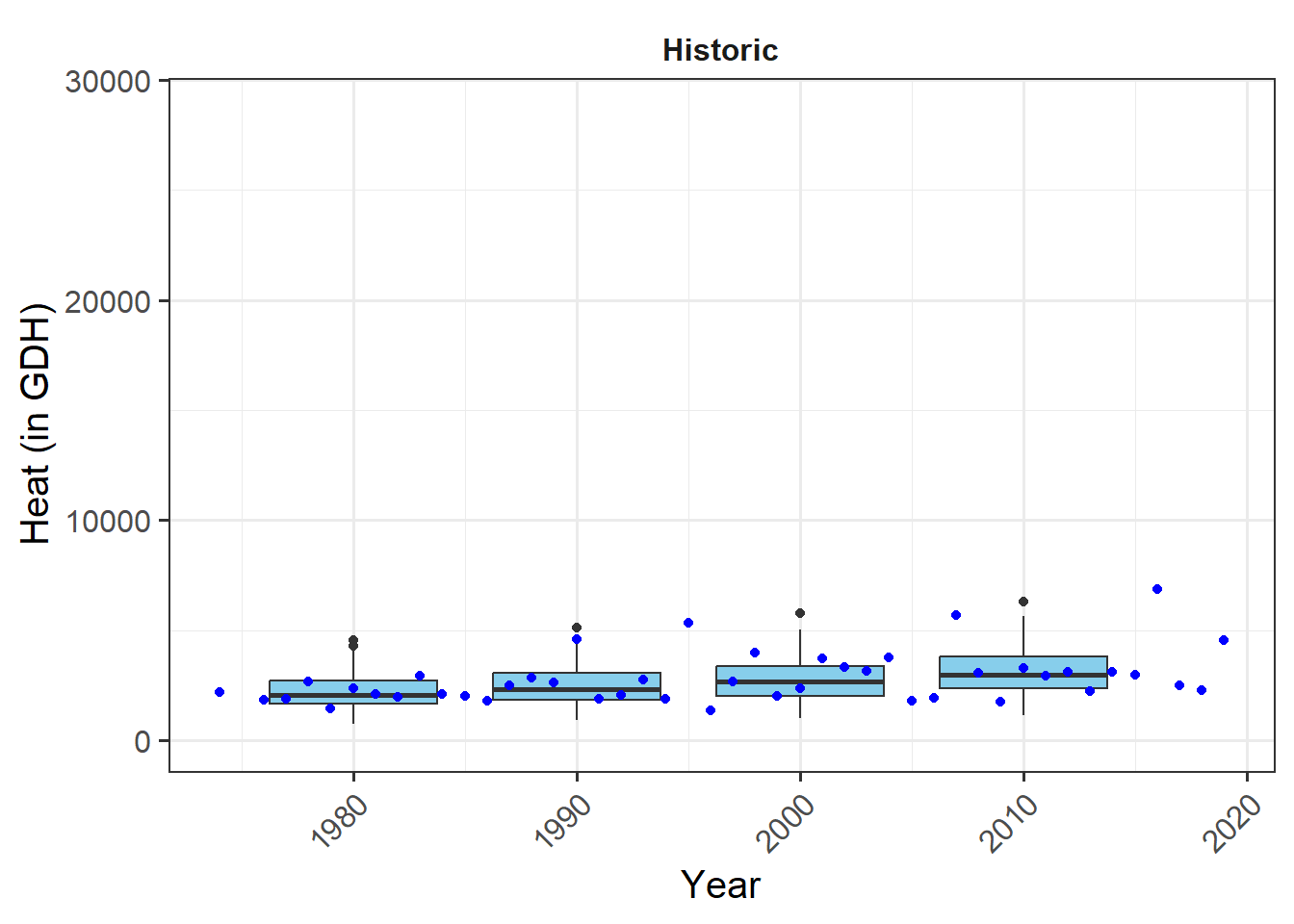
This is now pretty clear, and we can easily derive chilling and forcing phases. For these we can then calculate the mean chill accumulation and the mean heat accumulation, which approximate the respective requirements.
For reasons I’ll explain orally, I’m not using the mean of the chill and heat accumulation during the respective interval, but the median. I’ll use the 25% and 75% quantiles of the distributions as an estimate of uncertainty.
chill_phase<-c(290,10)
heat_phase<-c(17,97.5)

chill<-tempResponse(hourtemps = temps_hourly,
                    Start_JDay = chill_phase[1],
                    End_JDay = chill_phase[2],
                    models = list(Chill_Portions = Dynamic_Model),
                    misstolerance=10)

heat<-tempResponse(hourtemps = temps_hourly,
                    Start_JDay = heat_phase[1],
                    End_JDay = heat_phase[2],
                    models = list(GDH = GDH))
chill_requirement <- median(chill$Chill_Portions)
chill_req_error <- quantile(chill$Chill_Portions, c(0.25,0.75))

heat_requirement <- median(heat$GDH)
heat_req_error <- quantile(heat$GDH, c(0.25,0.75))
So we have a chilling requirement around 48.4 CP, but with a 50% confidence interval ranging from 34.4 to 59.1 CP. The heat need of this cultivar is estimated as 11870 GDH, with a 50% confidence interval ranging from 6625 to 16553 GDH.
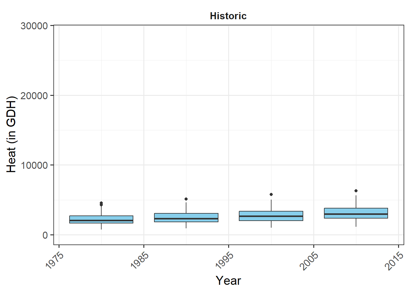
Let’s also look at the temperature range at this location in relation to the temperature sensitivity of the Dynamic Model.
Model_sensitivities_CKA<-
  Chill_model_sensitivity(latitude=50.6,
                          temp_models=list(Dynamic_Model=Dynamic_Model,GDH=GDH),
                          month_range=c(10:12,1:5))
write.csv(Model_sensitivities_CKA,
"data/Model_sensitivities_CKA.csv",row.names = FALSE)Chill_sensitivity_temps(Model_sensitivities_CKA,
weather_data,
temp_model="Dynamic_Model",
month_range=c(10,11,12,1,2,3),
legend_label="Chill per day \n(Chill Portions)") +
ggtitle("Chill model sensitivity at Klein-Altendorf on steroids")
This pattern looks a lot more promising. We see that temperature data spans quite a bit of model variation, which is an indication that PLS analysis may capture dormancy dynamics better than in the non-enhanced dataset from Klein-Altendorf.
Let’s see if we can see a pattern in the temperature response plot now.
pheno_trend_ggplot(temps=weather_data,
                   pheno=pheno_data[,c("Year","pheno")],
                   chill_phase=chill_phase,
                   heat_phase=heat_phase,
                   exclude_years=pheno_data$Year[is.na(pheno_data$pheno)],
                   phenology_stage="Bloom")
Now we can see a fairly clear temperature response pattern for Klein-Altendorf. Some of the points are still a bit off from what we would have liked to see. Here we should note that some of the treatments were quite far from what a tree might experience in an orchard. It seems likely that some of these extraordinary temperature curves were involved in generating strange patterns.
Exercises on experimental PLS
No exercises today. Maybe you can work on cleaning up your logbook.