Chapter 20 Simple phenology analysis
Learning goals for this lesson
- Understand why phenology modeling is tricky
- Appreciate the dangers of p-hacking
- Appreciate the importance of a causal theory in data analysis
20.1 Phenology analysis
Now we’ve finally reached the point in this module where we seriously start analyzing phenology. We’ll use the example of bloom dates of the pear cultivar Alexander Lucas that we already worked with in the frost analysis. As you may remember, we have a time series of first, full and last bloom dates recorded at Campus Klein-Altendorf between 1958 and 2019. For this analysis, I’ll just use the first bloom dates:
If you want to work with this example on your own computer, you can download the file here:
I suggest that you save this file in the data folder of your home directory: data/Alexander_Lucas_bloom_1958_2019.csv. Otherwise, you’ll have to adjust the path below. Note that the data are provided as a .csv file. To avoid any “comma vs. semicolon”-related problems, I recommend that you open it with the read_tab function.
Alex <- read_tab("data/Alexander_Lucas_bloom_1958_2019.csv")

Alex <- pivot_longer(Alex,
                     cols = c(First_bloom:Last_bloom),
                     names_to = "Stage",
                     values_to = "YEARMODA")

Alex_first <- Alex %>%
  mutate(Year = as.numeric(substr(YEARMODA, 1, 4)),
         Month = as.numeric(substr(YEARMODA, 5, 6)),
         Day = as.numeric(substr(YEARMODA, 7, 8))) %>%
  make_JDay() %>%
  filter(Stage == "First_bloom")
20.2 Time series analysis
The first analysis people often do with such a dataset is a simple analysis over time. Let’s first plot the data:
ggplot(Alex_first,
       aes(Pheno_year,
           JDay)) +
  geom_point() +
  ylab("First bloom date (day of the year)") +
  xlab ("Year") +
  theme_bw(base_size = 15)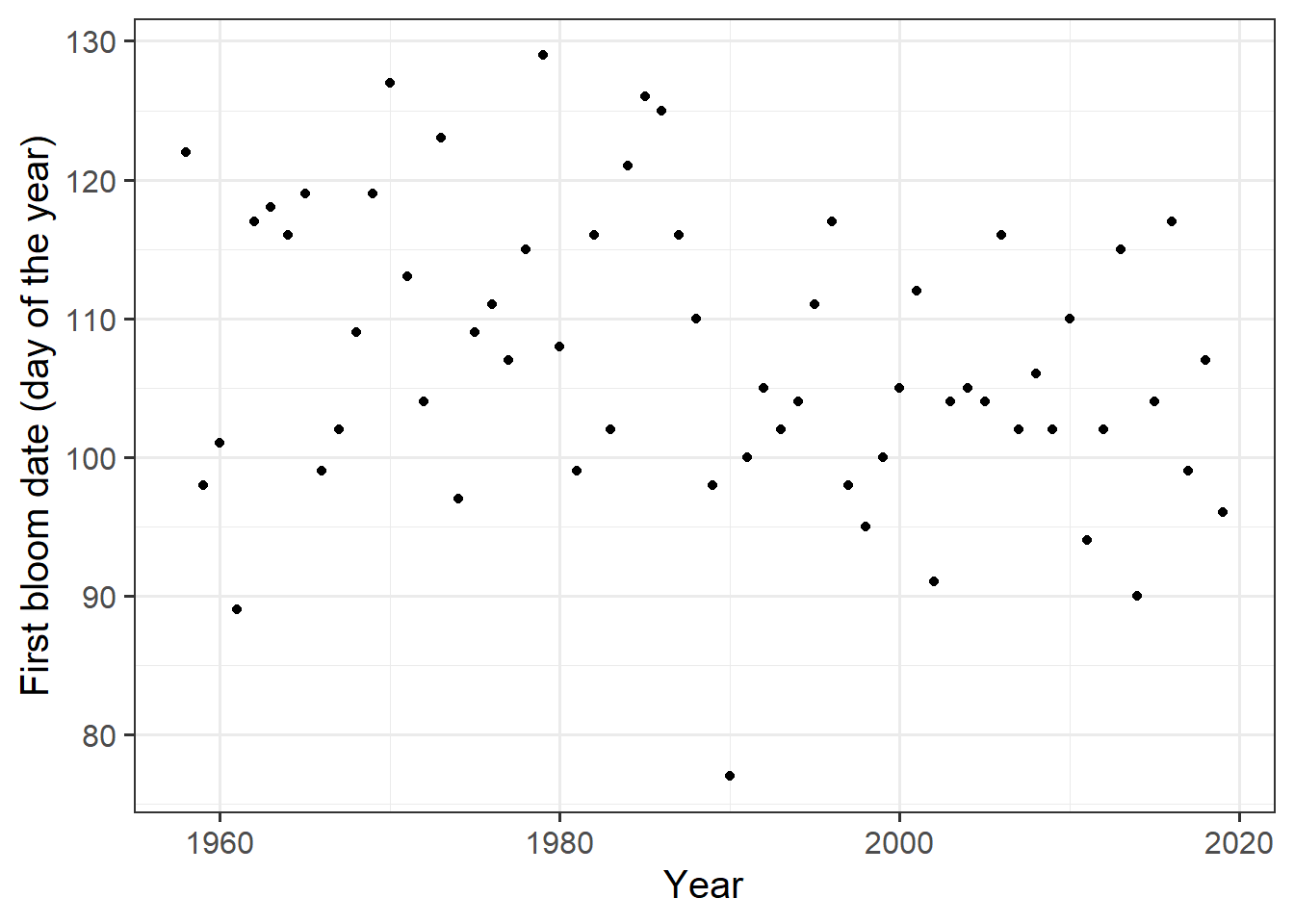
It’s a bit hard to see a clear pattern here, but let’s check if there is a trend over time. We’ve already encountered the Kendall test in an earlier lesson, and we can also apply this here:
## Warning: package 'Kendall' was built under R version 4.3.2## tau = -0.186, 2-sided pvalue =0.03533I’m getting a p-value of 0.035. The tau value is negative, so it seems we have a significant trend towards earlier bloom.
To determine how strong this trend is, many researchers use regression analysis, with model coefficients fitted to data. Let’s try this. We first assume a linear relationship between time and bloom dates: \[Bloomdate = a \cdot Phenoyear + b\]
To make the code easier to read, I’ll name the Pheno_year x and the Bloom date (JDay) y. I’ll also plot the data using ggplot:
##
## Call:
## lm(formula = y ~ x)
##
## Residuals:
##      Min       1Q   Median       3Q      Max
## -30.0959  -6.3591  -0.5959   6.6468  20.1238
##
## Coefficients:
##              Estimate Std. Error t value Pr(>|t|)
## (Intercept) 429.16615  142.06000   3.021   0.0037 **
## x            -0.16184    0.07144  -2.266   0.0271 *
## ---
## Signif. codes:  0 '***' 0.001 '**' 0.01 '*' 0.05 '.' 0.1 ' ' 1
##
## Residual standard error: 10.07 on 60 degrees of freedom
## Multiple R-squared:  0.0788, Adjusted R-squared:  0.06345
## F-statistic: 5.133 on 1 and 60 DF, p-value: 0.0271ggplot(Alex_first,
aes(Year,
JDay)) +
geom_point() +
geom_smooth(method = 'lm',
formula = y ~ x) +
ylab("First bloom date (day of the year)") +
xlab ("Year") +
theme_bw(base_size = 15)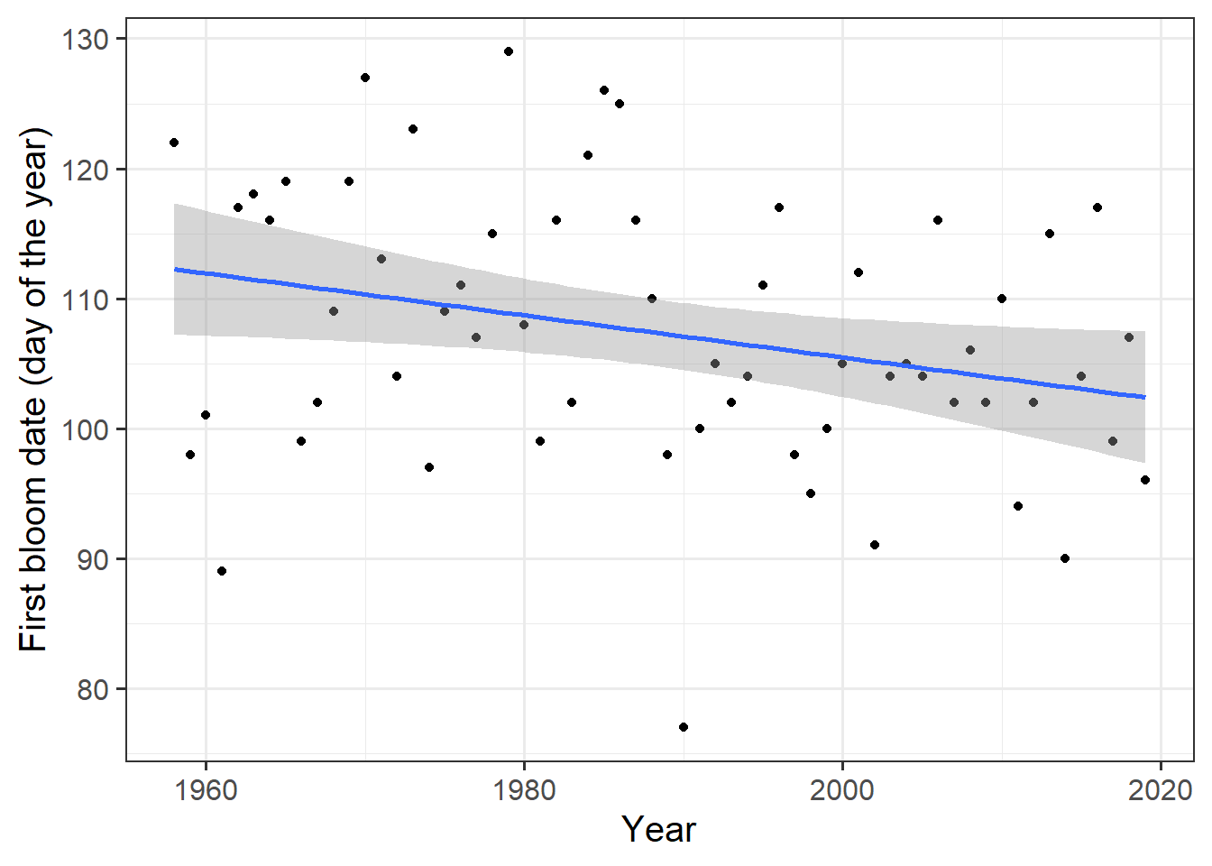
If you examine the outputs carefully, you’ll see that we’re getting a best estimate for the slope of -0.16. We also get a p-value here, but for a time series we’re better off using the one returned by the Kendall test. If you look at the diagram, you’ll notice that many of the data points are still pretty far from the regression line, with many of them way outside the confidence interval that is shown.
Maybe we can find another model that better describes the data. Many people would now start on a process of gradually making the model more complex, e.g. by fitting a second-order polynomial, or maybe a third-order polynomial… Let’s cut this process short and immediately fit a 25th-order polynomial:
##
## Call:
## lm(formula = y ~ poly(x, 25))
##
## Residuals:
##      Min       1Q   Median       3Q      Max
## -13.7311  -4.5098  -0.1227   2.8640  15.4590
##
## Coefficients:
##               Estimate Std. Error t value             Pr(>|t|)
## (Intercept)   107.3387     1.0549 101.753 < 0.0000000000000002 ***
## poly(x, 25)1  -22.8054     8.3063  -2.746              0.00937 **
## poly(x, 25)2   -5.8672     8.3063  -0.706              0.48451
## poly(x, 25)3   14.7725     8.3063   1.778              0.08377 .
## poly(x, 25)4   -5.3974     8.3063  -0.650              0.51995
## poly(x, 25)5  -11.6801     8.3063  -1.406              0.16825
## poly(x, 25)6    2.1928     8.3063   0.264              0.79329
## poly(x, 25)7   -0.3034     8.3063  -0.037              0.97107
## poly(x, 25)8    6.0115     8.3063   0.724              0.47391
## poly(x, 25)9  -22.2895     8.3063  -2.683              0.01094 *
## poly(x, 25)10   5.9522     8.3063   0.717              0.47825
## poly(x, 25)11  -6.1217     8.3063  -0.737              0.46590
## poly(x, 25)12   3.2676     8.3063   0.393              0.69636
## poly(x, 25)13 -14.8467     8.3063  -1.787              0.08229 .
## poly(x, 25)14  13.5180     8.3063   1.627              0.11237
## poly(x, 25)15  10.1544     8.3063   1.222              0.22946
## poly(x, 25)16 -12.6116     8.3063  -1.518              0.13767
## poly(x, 25)17  -1.3315     8.3063  -0.160              0.87354
## poly(x, 25)18  -6.3438     8.3063  -0.764              0.45000
## poly(x, 25)19  14.9753     8.3063   1.803              0.07978 .
## poly(x, 25)20   3.4573     8.3063   0.416              0.67972
## poly(x, 25)21 -29.1997     8.3063  -3.515              0.00121 **
## poly(x, 25)22  10.4145     8.3063   1.254              0.21799
## poly(x, 25)23   2.9898     8.3063   0.360              0.72100
## poly(x, 25)24 -14.3045     8.3063  -1.722              0.09363 .
## poly(x, 25)25 -20.9324     8.3063  -2.520              0.01631 *
## ---
## Signif. codes:  0 '***' 0.001 '**' 0.01 '*' 0.05 '.' 0.1 ' ' 1
##
## Residual standard error: 8.306 on 36 degrees of freedom
## Multiple R-squared:  0.6237, Adjusted R-squared:  0.3623
## F-statistic: 2.386 on 25 and 36 DF, p-value: 0.008421ggplot(Alex_first,
aes(Year,
JDay)) +
geom_point() +
geom_smooth(method='lm',
formula = y ~ poly(x, 25)) +
ylab("First bloom date (day of the year)") +
xlab ("Year") +
theme_bw(base_size = 15)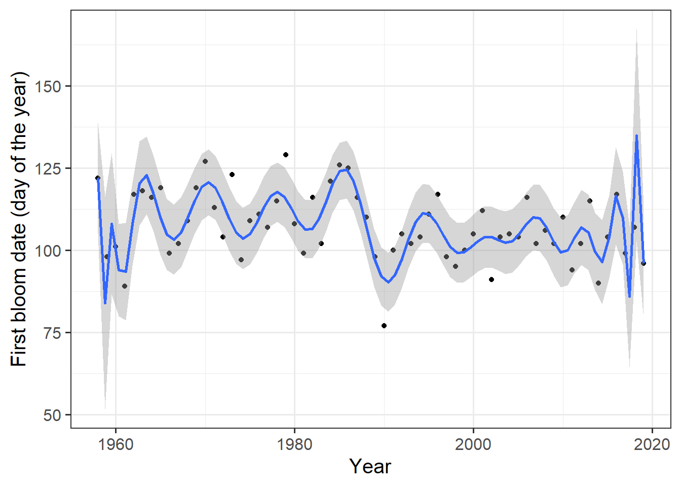
It’s a bit hard now of course to make a clear statement about the temporal trend, since there is no single number for the slope. The slope varies over time, but it can be calculated by taking the first derivative of the complex 25th-order polynomial we computed. But we got a stellar p-value, and almost all of the data points are contained in the confidence interval!
It’s probably obvious to you that this is not a useful model. If we make the model equation increasingly more complex, we’ll eventually find a structure that can perfectly fit all data points. This is not desirable, however, because we have no reason to expect that there is such a perfect relationship between our independent and dependent variables. Each measurement (such as a bloom date recording) comes with an error, and, more importantly, there may also be other factors in addition to time that affect bloom dates. If we make our model more complex than we can reasonably expect the actual relationship to be, we run the risk of overfitting our model. This means that we may get a very good fit, but our regression equation isn’t very useful for explaining the actual process we’re trying to model.
In the case of our 25th-order polynomial, we’re obviously looking at an overfit. In many other cases, however, overfits aren’t quite so easy to detect. The scientific literature is full of studies where authors took the structure of their regression model far beyond what could be considered a reasonable description of the underlying process. Especially in the field of machine-learning, overfitting is a very serious risk, in particular where the learning engines are basically black boxes that the analysts may not even fully understand.
20.3 p-hacking
A concept that is closely related to overfitting and that also often occurs in machine-learning is that of p-hacking, also known as a fishing expedition. The idea behind these terms is that when you look at a sufficiently large dataset, with lots of variables, you’re bound to find correlations somewhere in this dataset, regardless of whether your data involves actual causal relationships. Screening large datasets for ‘significant’ relationships and then presenting these as meaningful correlations is bad scientific practice (Nuzzo, 2014)! Possibly, such screening can lead to hypotheses that can then be tested through further studies, but we should not rely on this to generate ‘facts’.
20.4 The process that generates the data
Many researchers are focused on finding structure in the datasets they work with. While this can often produce useful insights, it can also lead to us neglecting an arguably more important objective of science - to find out how things work! What we really want to understand is the process that generates the data, rather than the data themselves.
While this argument may seem like semantics, it involves a change in perspective that can have important implications for how we do research. Rather than digging straight into the numbers, we first need to sit back and think about what may actually be going on in the system we’re analyzing. We can then use causal diagrams to sketch out how we think our system works:
\[A \to B\] With this realization, we quickly come to the conclusion that our analysis so far has been a bit beside the point.
Up to now, we were looking for the following relationship:
\[Time \to Phenology\] Can this possibly be what’s going on here? Can time drive phenology? While I won’t completely rule out that trees are somehow able to track the passage of time within their annual cycle, I’m pretty sure they have no idea what the current year is…
20.5 An ecological theory to guide our analysis
Before we start on an analysis of the kind we’re dealing with here, we should have a theory of what’s going on. In this case, this would be an ecological theory about what drives tree phenology. Let’s start with a very simple theory: Temperature drives phenology. I guess we already knew this, but it may still be useful to state it explicitly:
\[Temperature \to Phenology\] As you can see, this theory doesn’t involve time. The reason why we were able to find statistical relationships earlier is not that time (as in the calendar year) actually affects phenology - it is that temperatures have been rising over the years, mainly in response to anthropogenic global warming.
\[Time \to Temperature\] Well, actually this is \[Time \to GreenhouseGasEmissions \to ClimateForcing \to Temperature\] Since temperature, especially at the local scale, is subject to considerable random variation, this relationship may not be particularly strong. The noise in this relationship can easily keep us from detecting the actual response of tree phenology during our time series.
The full causal diagram of these three variables (without the greenhouse effect part) is \[Time \to Temperature \to Phenology\]
Sometimes we have no data on the intermediate steps in such a diagram. In such cases, we either have to live with a model that doesn’t actually get to the direct causal mechanisms in play, or we have to get a bit more creative with our analysis. Fortunately, here we actually do have data on temperature, so we can focus on the direct causal relationship between temperature and phenology.
20.6 Temperature correlations
Now that we clarified that it would make more sense to narrow in on the temperature-phenology relationship, we gained some conceptual clarity, but we are faced with a much greater statistical challenge. In correlating years with bloom dates, we had just two series of numbers to look at, since we had exactly one bloom date per year. Temperature, in contrast, is a variable we can measure at different temporal scales. If we just look at the average annual temperature, the statistical challenge is similar to using just the year number. Let’s see if we can find a correlation for this. You may have to click the button to download weather data first. I’d suggest you save it then under data/TMaxTMin1958-2019_patched.csv.
temperature <- read_tab("data/TMaxTMin1958-2019_patched.csv")

Tmin <- temperature %>%
  group_by(Year) %>%
  summarise(Tmin = mean(Tmin))

Tmax <- temperature %>%
  group_by(Year) %>%
  summarise(Tmax = mean(Tmax))

Annual_means <- Tmin %>%
  cbind(Tmax[,2]) %>%
  mutate(Tmean = (Tmin + Tmax)/2)

Annual_means <- merge(Annual_means,
                      Alex_first)

Annual_means_longer <- Annual_means[,c(1:4,10)] %>%
  pivot_longer(cols = c(Tmin:Tmean),
               names_to = "Variable",
               values_to = "Temp")

ggplot(Annual_means_longer,
       aes(x=Temp,
           y=JDay)) +
  geom_point() +
  geom_smooth(method="lm",
              formula=y~x) +
  facet_wrap("Variable")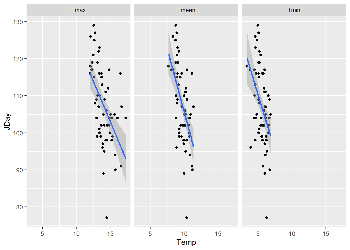
##
## Call:
## lm(formula = Annual_means$JDay ~ Annual_means$Tmin)
##
## Residuals:
##      Min       1Q   Median       3Q      Max
## -25.4960  -6.9227  -0.0472   6.9066  18.4940
##
## Coefficients:
##                   Estimate Std. Error t value             Pr(>|t|)
## (Intercept)        140.288      8.610  16.293 < 0.0000000000000002 ***
## Annual_means$Tmin   -6.020      1.558  -3.864             0.000277 ***
## ---
## Signif. codes:  0 '***' 0.001 '**' 0.01 '*' 0.05 '.' 0.1 ' ' 1
##
## Residual standard error: 9.385 on 60 degrees of freedom
## Multiple R-squared:  0.1992, Adjusted R-squared:  0.1859
## F-statistic: 14.93 on 1 and 60 DF, p-value: 0.0002765##
## Call:
## lm(formula = Annual_means$JDay ~ Annual_means$Tmax)
##
## Residuals:
## Min 1Q Median 3Q Max
## -28.2420 -5.7340 0.3032 5.8515 19.4918
##
## Coefficients:
## Estimate Std. Error t value Pr(>|t|)
## (Intercept) 168.5020 12.9573 13.004 < 0.0000000000000002 ***
## Annual_means$Tmax -4.3586 0.9198 -4.739 0.0000136 ***
## ---
## Signif. codes: 0 '***' 0.001 '**' 0.01 '*' 0.05 '.' 0.1 ' ' 1
##
## Residual standard error: 8.947 on 60 degrees of freedom
## Multiple R-squared: 0.2723, Adjusted R-squared: 0.2602
## F-statistic: 22.45 on 1 and 60 DF, p-value: 0.00001363##
## Call:
## lm(formula = Annual_means$JDay ~ Annual_means$Tmean)
##
## Residuals:
## Min 1Q Median 3Q Max
## -25.9808 -5.5032 0.3793 6.1267 18.1822
##
## Coefficients:
## Estimate Std. Error t value Pr(>|t|)
## (Intercept) 173.467 12.379 14.013 < 0.0000000000000002
## Annual_means$Tmean -6.780 1.264 -5.363 0.00000138
##
## (Intercept) ***
## Annual_means$Tmean ***
## ---
## Signif. codes: 0 '***' 0.001 '**' 0.01 '*' 0.05 '.' 0.1 ' ' 1
##
## Residual standard error: 8.623 on 60 degrees of freedom
## Multiple R-squared: 0.324, Adjusted R-squared: 0.3128
## F-statistic: 28.76 on 1 and 60 DF, p-value: 0.000001381There’s a relationship here, but this is still not really a convincing analysis. The main reason is that the time period we’re calculating the mean temperatures for is the whole year, even though bloom already occurs in spring. Temperatures after this can’t possibly affect the bloom date in the year of interest! Then why did we get such convincing results, with exceptionally low p values? Again, the reason is climate change. Temperatures have been rising over time, and phenology has advanced over time, so later years generally feature earlier bloom dates. To get to an analysis that has a chance of actually reflecting a causal relationship, however, we need to restrict the analysis to a range of dates that can plausibly affect bloom dates.
Let’s write a quick function to screen for such correlations. To facilitate this, we’ll use JDay, i.e. the day of the year, to express the date.
temps_JDays <-
  make_JDay(temperature)

corr_temp_pheno <- function(start_JDay, # the start JDay of the period
                            end_JDay, # the start JDay of the period
                            temps_JDay = temps_JDays, # the temperature dataset
                            bloom = Alex_first) # a data.frame with bloom dates
{
  temps_JDay <- temps_JDay %>%
    mutate(Season = Year)

  if(start_JDay > end_JDay)
    temps_JDay$Season[temps_JDay$JDay >= start_JDay]<-
      temps_JDay$Year[temps_JDay$JDay >= start_JDay]+1

  if(start_JDay > end_JDay)
    sub_temps <- subset(temps_JDay,
                        JDay <= end_JDay | JDay >= start_JDay)

  if(start_JDay <= end_JDay)
    sub_temps <- subset(temps_JDay,
                        JDay <= end_JDay & JDay >= start_JDay)

  mean_temps <- sub_temps %>%
    group_by(Season) %>%
    summarise(Tmin = mean(Tmin),
              Tmax = mean(Tmax)) %>%
    mutate(Tmean = (Tmin + Tmax)/2)

  colnames(mean_temps)[1] <- c("Pheno_year")

  temps_bloom <- merge(mean_temps,
                       bloom[c("Pheno_year",
                               "JDay")])

  # Let's just extract the slopes of the regression model for now
  slope_Tmin <- summary(lm(temps_bloom$JDay~temps_bloom$Tmin))$coefficients[2,1]
  slope_Tmean <- summary(lm(temps_bloom$JDay~temps_bloom$Tmean))$coefficients[2,1]
  slope_Tmax <- summary(lm(temps_bloom$JDay~temps_bloom$Tmax))$coefficients[2,1]

  c(start_JDay = start_JDay,
    end_JDay = end_JDay,
    length = length(unique(sub_temps$JDay)),
    slope_Tmin = slope_Tmin,
    slope_Tmean = slope_Tmean,
    slope_Tmax = slope_Tmax)
}

corr_temp_pheno(start_JDay = 305,
                end_JDay = 29,
                temps_JDay = temps_JDays,
                bloom = Alex_first)
## start_JDay end_JDay length slope_Tmin slope_Tmean
## 305.000000 29.000000 91.000000 -1.821312 -2.135616
## slope_Tmax
## -2.237499## start_JDay end_JDay length slope_Tmin slope_Tmean
## 305.000000 45.000000 107.000000 -2.254426 -2.655599
## slope_Tmax
## -2.799758Now we can apply this function to all combinations of days we we find reasonable. Rather than trying all possible values, I’ll only use every 5th possible start and end date (that’s already enough computing work).
library(colorRamps) # for the color scheme we'll use in the plot

stJDs <- seq(from = 1,
             to = 366,
             by = 10)

eJDs <- seq(from = 1,
            to = 366,
            by = 10)

for(stJD in stJDs)
  for(eJD in eJDs)
    {correlations <- corr_temp_pheno(stJD,
                                     eJD)

    if(stJD == 1 & eJD == 1)
      corrs <- correlations else
        corrs <- rbind(corrs, correlations)
}


slopes <- as.data.frame(corrs) %>%
  rename(Tmin = slope_Tmin,
         Tmax = slope_Tmax,
         Tmean = slope_Tmean) %>%
  pivot_longer(cols = c(Tmin : Tmax),
               values_to = "Slope",
               names_to = "Variable")

ggplot(data = slopes,
       aes(x = start_JDay,
           y = length,
           fill = Slope)) +
  geom_tile() +
  facet_wrap(vars(Variable)) +
  scale_fill_gradientn(colours = matlab.like(15)) +
  ylab("Interval duration (days)") +
  xlab("Start date of temperature summary interval (Day of year)") +
  theme_bw(base_size = 15)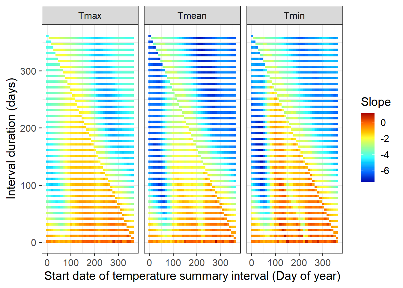
While this plot can give us an idea about the periods during which temperatures are strongly related to bloom dates, we’ve actually veered slightly off track again. First, if we now went for the strongest possible influence and declared this as the main driver of bloom dates, we’d be p-hacking again. More importantly, we’re again looking for something that’s a bit different from what we should actually expect based on our ecological knowledge.
We learned earlier that bloom dates are determined by two separate temperature-dependent processes: chilling and forcing. So we need more than one temperature period! We could now expand our p-hacking exercise to include multiple temperature summary variables. We could then also apply multiple regression, which can automatically identify variables that are correlated with bloom dates.
Such fishing for correlations is a tedious and unsatisfying exercise, and it wouldn’t seem particularly enlightened. It’s likely to lead to overfits, and it can easily miss important temperature response periods by narrowing in on the phases that are most strongly correlated to the outcome variable. So let’s not do this and instead take a step back again to think about the theory. Here’s what we should actually expect:
\[\substack{Temp_{chilling} \to chill \to\\ Temp_{forcing} \to heat \to} BloomDate\] We could now start developing equations that describe what we think we know about chilling and forcing. Many colleagues have done this and then fitted the equations they came up with to observed phenology data. I don’t want to go into the details here, but I want to point out that most of the chill models we compared in the last lesson come from such exercises. Some of these are clearly way off the mark - and I assume the phenology models they were a part of still did pretty well. This is possible, because most phenology models have quite a few parameters, e.g. the start and end dates of chilling and forcing periods, the chilling and forcing requirements and the specifications of the temperature response curves during both phases. It’s easy for these parameters to compensate for each other, so that we get the right result for the wrong reasons. Such models have also often been fitted through trial and error or through less-than-convincing machine learning algorithms.
So before we build a model, let’s see if we can find a bit more information to work with. In the next lesson, we’ll combine our ecological knowledge with a machine learning technique to figure out when trees are responsive to temperature.
Exercises on simple phenology analysis
Please document all results of the following assignments in your learning logbook.
We’re not going to practice any of the analyses we’ve seen in this lesson, because I don’t find them particularly useful…
- Provide a brief narrative describing what p-hacking is, and why this is a problematic approach to data analysis.
- Provide a sketch of your causal understanding of the relationship between temperature and bloom dates.
- What do we need to know to build a process-based model from this?